Floods Data Pathfinder

Floods affect more people than any other type of natural disaster. This data pathfinder links to NASA datasets and tools that can aid with decisions regarding flood response and mitigation.
Image
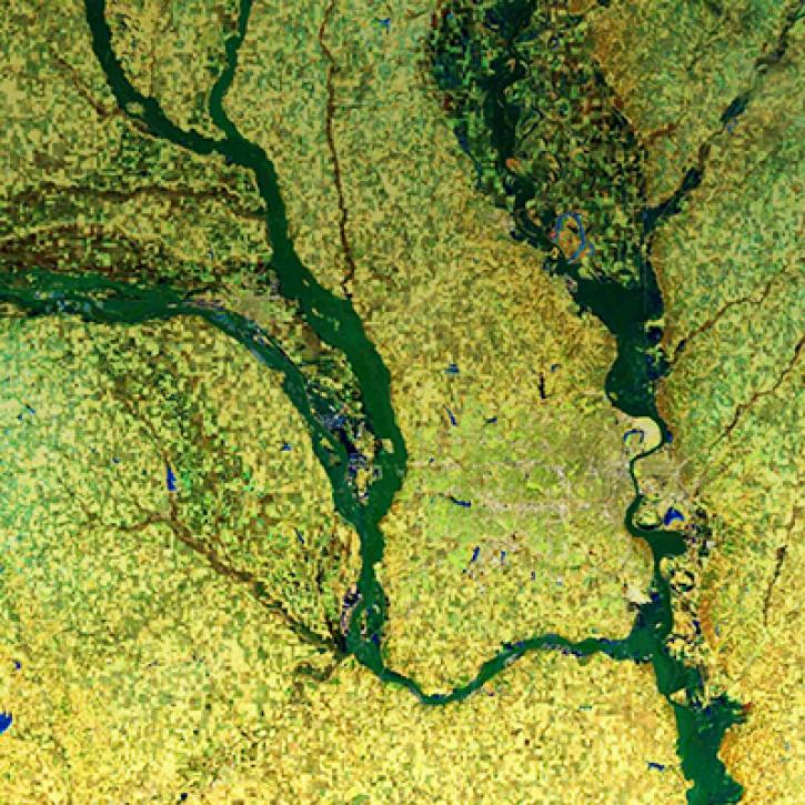
Two days of heavy rain, May 2020, led to catastrophic dam failures and major flooding in Midland County, Michigan. The natural-color image is from Landsat's Operational Land Imager.
Heavy rain in May 2020 led to catastrophic dam failures and major flooding in Midland County, Michigan. Natural-color image from Landsat's Operational Land Imager. Credit: NASA Earth Observatory

Floods affect more people than any other type of natural disaster and the number of flood-related disasters is increasing at an alarming rate, resulting in major social and economic losses. The United Nations, in its Sustainable Development Goals, has called for a transition from just responding to flood events to actually assessing the vulnerability, exposure, and risk of communities with the ultimate goal of mitigating potential devastating impacts.

Scientists and decision makers, using satellite- and ground-based data as well as models, can evaluate the factors which contribute to an area's predisposition to flooding, including precipitation, soil moisture, and topography. They can use satellite data to monitor inundation and respond to events in near real-time.

Please visit the Earthdata Forum, where you can interact with other users and NASA subject matter experts on a variety of Earth science research and applications topics.

Find the Data

Many environmental variables, such as precipitation, soil moisture, snow cover, etc. contributed to natural flood event.
Flood events can have drastic economic and social losses to communities. NASA measurements can be used to map flood inundation and to understand vulnerability and exposure of communities to aid with disaster relief efforts.
Tools for Data Access and Visualization

Earthdata Search | Panoply | Giovanni | Worldview | AppEEARS | Soil Moisture Visualizer | MODIS/VIIRS Subsetting Tools Suite | Spatial Data Access Tool (SDAT)| Sentinel Toolbox

Earthdata Search

Earthdata Search is a tool for data discovery of Earth Observation data collections from NASA's Earth Observing System Data and Information System (EOSDIS), as well as U.S and international agencies across the Earth science disciplines. Users (including those without specific knowledge of the data) can search for and read about data collections, search for data files by date and spatial area, preview browse images, and download or submit requests for data files, with customization for select data collections.


Screenshot of the Search Earthdata site.

In the project area, for some datasets, you can customize your granule. You can reformat the data and output as HDF, NetCDF, ASCII, KML, or a GeoTIFF. You can also choose from a variety of projection options. Lastly, you can subset the data, obtaining only the bands that are needed.


Earthdata Search customization tools diagram.

Panoply

HDF and NetCDF files can be viewed in Panoply, a cross-platform application that plots geo-referenced and other arrays. Panoply offers additional functionality, such as slicing and plotting arrays, combining arrays, and exporting plots and animations.

Giovanni

Giovanni is an online environment for the display and analysis of geophysical parameters. There are many options for analysis. The following are the more popular ones.

  • Time-averaged maps are a simple way to observe the variability of data values over a region of interest.
  • Map animations are a means to observe spatial patterns and detect unusual events over time.
  • Area-averaged time series are used to display the value of a data variable that has been averaged from all the data values acquired for a selected region for each time step.
  • Histogram plots are used to display the distribution of values of a data variable in a selected region and time interval.

For more detailed tutorials:

  • Giovanni How-To's on GES DISC's YouTube channel.
  • Data recipe for downloading a Giovanni map as NetCDF and converting its data to quantifiable map data in the form of latitude-longitude-data value ASCII text.

Worldview

NASA's EOSDIS Worldview visualization application provides the capability to interactively browse over 1,000 global, full-resolution satellite imagery layers and then download the underlying data. Many of the available imagery layers are updated within three hours of observation, essentially showing the entire Earth as it looks "right now." This supports time-critical application areas such as wildfire management, air quality measurements, and flood monitoring. Imagery in Worldview is provided by NASA's Global Imagery Browse Services (GIBS). Worldview now includes nine geostationary imagery layers from GOES-East, GOES-West and Himawari-8 available at ten minute increments for the last 30 days. These layers include Red Visible, which can be used for analyzing daytime clouds, fog, insolation, and winds; Clean Infrared, which provides cloud top temperature and information about precipitation; and Air Mass RGB, which enables the visualization of the differentiation between air mass types (e.g., dry air, moist air, etc.). These full disk hemispheric views allow for almost real-time viewing of changes occurring around most of the world.


Image
Worldview data visualization of the nighttime lights in Puerto Rico pre- and post- Hurricane Maria, which made landfall on September 20, 2017. Post-hurricane image shows widespread outages around San Juan, including key hospital and transportation infrastructure.
Worldview Suomi NPP/VIIRS nighttime lights comparison image showing power outages caused by Hurricane Irma in September 2017. The right image (acquired 1 September 2017) shows the island before Hurricane Irma. The left image (acquired 9 September 2017) shows power outages across island after Hurricane Irma. NASA Worldview image.

AppEEARS

AppEEARS, from LP DAAC, offers a simple and efficient way to access and transform geospatial data from a variety of federal data archives. AppEEARS enables users to subset geospatial datasets using spatial, temporal, and band/layer parameters. Two types of sample requests are available: point samples for geographic coordinates and area samples for spatial areas via vector polygons.

Performing Area Extractions

After choosing to request an area extraction, you will be taken to the Extract Area Sample page where you will specify a series of parameters that are used to extract data for your area(s) of interest.

Spatial Subsetting

Define your region of interest in one of these three ways:

  • Upload a vector polygon file in shapefile format (you can upload a single file with multiple features or multipart single features). The .shp, .shx, .dbf, or .prj files must be zipped into a file folder to upload.
  • Upload a vector polygon file in GeoJSON format (can upload a single file with multiple features or multipart single features).
  • Draw a polygon on the map by clicking on the Bounding box or Polygon icons (single feature only).

Select the date range for your time period of interest.

Specify the range of dates for which you wish to extract data by entering a start and end date (MM-DD-YYYY) or by clicking on the Calendar icon and selecting dates a start and end date in the calendar.

Adding Data Layers

Enter the product short name (e.g., MOD09A1, ECO3ETPTJPL), keywords from the product long name, a spatial resolution, a temporal extent, or a temporal resolution into the search bar. A list of available products matching your query will be generated. Select the layer(s) of interest to add to the Selected layers list. Layers from multiple products can be added to a single request. Be sure to read the list of available products available through AppEEARS.

Image
Appeears_Flood.

Selecting Output Options

Two output file formats are available:

  • GeoTIFF
  • NetCDF-4

If GeoTIFF is selected, one GeoTIFF will be created for each feature in the input vector polygon file for each layer by observation. If NetCDF-4 is selected, outputs will be grouped into .nc files by product and by feature.


If GeoTIFF is selected, you must select a projection

Interacting with Results

Once your request is completed, from the Explore Requests page, click the View icon in order to view and interact with your results. This will take you to the View Area Sample page.

The Layer Stats plot provides time series boxplots for all of the sample data for a given feature, data layer, and observation. Each input feature is renamed with a unique AppEEARS ID (AID). If your feature contains attribute table information, you can view the feature attribute table data by clicking on the Information icon to the right of the Feature dropdown. To view statistics from different features or layers, select a different AID from the Feature dropdown and/or a different layer of interest from the Layer dropdown.


Interpreting Results in AppEEARS

Be sure to check out the AppEEARS documentation to learn more about downloading the output GeoTIFF or NetCDF-4 files.

Soil Moisture Visualizer

ORNL DAAC has developed a Soil Moisture Visualizer tool (read about it at Soil Moisture Data Sets Become Fertile Ground for Applications) that integrates a variety of different soil moisture datasets over North America. The visualization tool incorporates in-situ, airborne, and remote sensing data into one easy-to-use platform. This integration helps to validate and calibrate the data, and provides spatial and temporal data continuity. It also facilitates exploratory analysis and data discovery for different groups of users. The Soil Moisture Visualizer offers the capability to geographically subset and download time series data in .csv format. For more information on the available datasets and use of the visualizer, view the Soil Moisture Visualizer Guide.

To use the visualizer, select a dataset of interest under Data. Depending on the dataset chosen, the visualizer provides the included latitude/longitude or an actual site location name and relative time frames of data collection. Upon selection of the parameter, the tool displays a time series with available datasets. All measurements are volumetric soil moisture. Surface soil moisture is the daily average of measurements at 0-5 cm depth, and root zone soil moisture (RZSM) is the daily average of measurements at 0-100 cm depth. Lastly it provides data sources for download.


Image
ORNL DAAC Soil Moisture Visualizer
The Soil Moisture Visualizer allows users to compare soil moisture measurements from multiple sources (figure legends, top left and bottom right) at the same location. In this screenshot, Level 4 Root Zone Soil Moisture (L4 RZSM) data from NASA’s Soil Moisture Active Passive (SMAP) Observatory are shown with data from in situ sensors across the 9-kilometer Equal-Area Scalable Earth (EASE) grid cell encompassing the Tonzi Ranch Fluxnet site in the Sierra Nevada foothills of California. Daily precipitation values for the site (purple spikes) are also provided for reference.

MODIS/VIIRS Subsetting Tools Suite

ORNL DAAC also has several MODIS and VIIRS Subset Tools for subsetting data.

  • With the Global Subset Tool, you can request a subset for any location on earth, provided as GeoTIFF and in text format, including interactive time-series plots and more. Users specify a site by entering the site's geographic coordinates and the area surrounding that site, from one pixel up to 201 x 201 km. From the available datasets, you can specify a date and then select from MODIS Sinusoidal Projection or Geographic Lat/Long. You will need an Earthdata Login to request data.
  • With the Fixed Subsets Tool, you can download pre-processed subsets for 3000+ field and flux tower sites for validation of models and remote sensing products. The goal of the Fixed Sites Subsets Tool is to prepare summaries of selected data products for the community to characterize field sites. It includes sites from networks such as NEON, ForestGeo, PhenoCam and LTER that are of relevance to the biodiversity community.
  • With the Web Service, you can retrieve subset data (in real-time) for any location(s), time period, and area programmatically using a REST web service. Web service client and libraries are available in multiple programming languages, allowing integration of subsets into users' workflow.


Image
Directions for subsetting data with the ORNL DAAC MODIS and VIIRS subset tool
Top image: The Global Subsets Tool enables users to download available products for any location on Earth. Bottom image: The Fixed Sites Subsets Tool provides spatial subsets for established field sites for site characterization and validation of models and remote sensing products.

Spatial Data Access Tool (SDAT)

ORNL DAAC's SDAT is an Open Geospatial Consortium standards-based web application to visualize and download spatial data in various user-selected spatial/temporal extents, file formats, and projections. Several datasets including land cover, biophysical properties, elevation, and selected ORNL DAAC archived data are available through SDAT. KMZ files are also provided for data visualization in Google Earth.

Within SDAT, select a dataset of interest. Upon selection, the map service will open displaying the various measurements, with the associated granule, and a visualization of the selected granule.


Image
Canopy Height, Kalimantan Forests, Indonesia, 2014 from the Oak Ridge National Laboratory Distributed Active Archive Center Spatial Data Access Tool.

You can then select your spatial extent, projection, and output format for downloading.


Image
Canopy Height, Kalimantan Forests, Indonesia, 2014 from the Oak Ridge National Laboratory Distributed Active Archive Center Spatial Data Access Tool with various output options.

Sentinel Toolbox

The European Space Agency's (ESA) Sentinel-1 Mission consists of two satellites, Sentinel-1A and Sentinel-1B, with SAR instruments operating at a C-Band frequency. They orbit 180° apart, together imaging the entire Earth every six days. SAR is an active sensor that can penetrate cloud cover and vegetation canopy, and also observe at night. Therefore, it is ideal for flood inundation mapping. It also provides useful information to detect movement of Earth material after an earthquake, volcanic eruption or landslide. SAR data are very complex to process, however, ESA has developed a Sentinel-1 Toolbox to aid with processing and analysis of Sentinel-1 data.

For more information on active sensors, see What is Remote Sensing? and for more information on SAR specifically, see What is SAR?.

Flood Inundation Mapping

Image
SARSignal

Before choosing data, it's important to determine which band meets your needs, as radar signals penetrate deeper as the sensor wavelength increases. This difference in penetration is due to the dielectric properties of a given medium, which dictate how much of the incoming radiation scatters at the surface, how much signal penetrates into the medium, and how much of the energy gets lost to the medium through absorption.

Another important parameter to take into consideration when choosing a dataset is the polarization, or the direction in which the signal is transmitted and/or received: horizontally or vertically. Dual polarization, for example, refers to two different signal directions, horizontal/vertical and vertical/horizontal (HV and VH). Knowing the polarization from which a SAR image was acquired is important, as signals at different polarizations interact differently with objects on the ground, affecting the recorded radar brightness in a specific polarization channel.


Image
Strong scattering in HH indicates a predominance of double-bounce scattering (e.g., stemmy vegetation, manmade structures), while strong VV relates to rough surface scattering (e.g., bare ground, water), and spatial variations in dual polarization indicate the distribution of volume scatterers (e.g., vegetation and high-penetration soil types such as sand or other dry porous soils).
Strong scattering in HH indicates a predominance of double-bounce scattering (e.g., stemmy vegetation, manmade structures), while strong VV relates to rough surface scattering (e.g., bare ground, water), and spatial variations in dual polarization indicate the distribution of volume scatterers (e.g., vegetation and high-penetration soil types such as sand or other dry porous soils). Credit: NASA SAR Handbook.

Once you have downloaded the needed SAR data, it must be calibrated to account for distortion in the data. The objective in performing calibration is to create an image where the value of each pixel is directly related to the backscatter of the surface. So calibration takes into account radiometric distortion, signal loss as the wave propagates, saturation, and speckle. This process is critical for analyzing images quantitatively; it is also important for comparing images from different sensors, modalities, processors, and different acquisition dates.


Screenshot of the Sentinel-1 toolbox

Important note: DO NOT unzip the downloaded SAR file. Open the .zip file from within the Sentinel Toolbox. When you expand the Bands folder, you will see an amplitude and an intensity file for each polarization option. (The intensity band is a virtual one and is the square of the amplitude.) Open the amplitude file. Subset the data by zooming in to the area of interest and right-clicking on "Spatial Subset from View."

Calibration is done by following these steps:

  1. Radiometric calibration is performed by selecting Radar/Radiometric/Calibration (leave parameters as default).
  2. Geometric correction is done next to fix the main geometric distortions, due to Slant Range, Layover, Shadow, and Foreshortening. Terrain correction can be performed by selecting Radar/Geometric/Terrain Correction/ Range-Doppler Terrain Correction. This requires a digital elevation model (within the processing parameters, SRTM is the default selection). You can also specify a map projection in the processing parameters.


Sentinel-1 Toolbox Geometric Correction

Another characteristic of SAR images that must be accounted for is speckle. Speckle is the grey level variation that occurs between adjacent resolution cells, creating a grainy texture. Within the Toolbox, speckle can be removed by selecting "Radar/Speckle Filtering/Single Product Speckle Filter," and then choosing a type of filter; "Lee" is one of the most common.


Comparison of speckle in SAR imagery within Sentinel-1 Toolbox

For further information on SAR flood inundation mapping, see ASF DAAC's flood inundation recipes for QGIS or ArcGIS.

Last Updated
Jul 15, 2021