Global sea level has risen by about 8 inches since reliable record keeping began in 1880 and is projected to rise another 1 to 8 feet by 2100. This Data Pathfinder provides links to NASA datasets and tools that can aid in our understanding of sea level change.
According to the United Nations, 40% of the world's population lives within 100 km of a coast, meaning that close to three billion people could be impacted by changes in sea level. Coastal communities are centers of economic, social, and cultural development; they also provide significant ecological and environmental services. Global Mean Sea Level (GMSL) is increasing at about 3.3 millimeters per year (mm/y) and is already having catastrophic effects in coastal communities through flooding, erosion, and storm-related hazards.
Thermal expansion and the addition of fresh water to oceans from glacier and ice sheet melt are causing a rise in GMSL. As the atmosphere warms, much of its heat gets absorbed by the ocean, causing the water to expand. More than 90% of warming over the past 50 years has occurred in the ocean. Along with this thermal expansion, land-based glaciers and ice sheets are melting. Greenland is losing about 289 gigatons (Gt) of ice per year and Antarctica about 132 Gt. To put this in perspective, the largest animal on Earth, a blue whale, weighs about 330,000 pounds or 165 tons; each year Earth loses the equivalent in ice of about 2.5 billion blue whales.
Locally and regionally, sea level change can be significantly different from the global average due to factors such as natural and human-induced subsidence (sinking or settling of the ground), ocean currents, and rebound from the compressive weight of Ice Age glaciers.
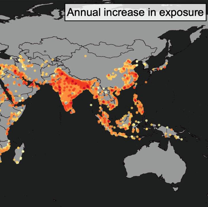
Exposure and vulnerability are important components in risk-management efforts and adaptation strategies. The presence of people, animals and ecosystems, environmental resources, infrastructure, or economic, social, and cultural assets in places and settings that could be adversely affected by a change in sea level is called exposure. Vulnerability is the propensity of a community to be adversely affected by sea level change, taking into consideration factors such as susceptibility to harm and lack of capacity to cope and adapt. Risk is determined by exposure and vulnerability to hazards.
Our current scientific understanding of sea level change is unprecedented due in large part to the long-term records of sea level and almost 30 years of satellite altimetry. NASA provides a wealth of data that support this understanding.
Please visit the Earthdata Forum, where you can interact with data users and NASA subject matter experts on a variety of Earth science research and applications topics.
About the Data
NASA collaborates with other federal entities and international space organizations, including NOAA, USGS, the Japan Aerospace Exploration Agency (JAXA) and Ministry of Economy, Trade, and Industry (METI), and the European Space Agency (ESA), to collect and distribute sea level data. Data from these agencies and various NASA instruments can be used for understanding a number of phenomena that contribute to sea level change. NASA also provides datasets to help assess the impacts, exposure, and vulnerability of individual communities to rising sea levels.
Datasets referenced in this Pathfinder are from the satellite and airborne sensors shown in the table below, including their spatial and temporal resolutions. Note that many satellites and platforms carry multiple sensors; the table below only lists the primary sensor used in collecting the specified measurement. When available, NASA's Land, Atmosphere Near real-time Capability for EOS (LANCE) provides data to the public generally within three hours of a satellite overpass, which allows for near real-time (NRT) monitoring and decision making (sensors from which select datasets are available in LANCE are marked with *).
Note: This is not an exhaustive list of datasets but rather only includes datasets from NASA's Earth Observing System Data and Information System (EOSDIS).
Measurement
Satellite
Sensor
Spatial Resolution
Temporal Resolution
Glacier Surface Elevation
NASA Oceans Melting Greenland (OMG) Airborne
Glacier and Land Ice Surface Topography Interferometer Airborne (GLISTIN-A) radar
3 m
Global Mean Sea Level, Sea Surface Height Anomalies
NASA Topographic Experiment (TOPEX)/Poseidon, Jason-1, Jason-2, Jason-3
In addition to mission data available through EOSDIS Distributed Active Archive Centers (DAACs), NASA has a series of environmental simulation models that use satellite- and ground-based observational data. There are a few reasons model data may be preferred over remote sensing observations, including obtaining more complex data parameters, temporal coverage, spatial coverage, and/or data completeness.
Models are often used for projections and forecasts, but time is not the only dimension in which projections can be made. Models can also project into space, offering data where sensors are unavailable. For instance, satellite observations of land surface temperatures can only be made where there is a clear view of the land. Clouds and dust can obscure views, and observations are further dependent on the type of land cover; highly reflective areas, such as snow and urban areas, can be challenging to observe. A model allows researchers to fill those gaps by bringing in additional data from ground stations or other sensors that measure different wavelengths.
The Modern-Era Retrospective analysis for Research and Applications, Version 2 (MERRA-2) model provides data beginning in 1980. Due to the amount of historical data available, MERRA-2 data can be used to look for trends and patterns as well as anomalies. As climate is typically measured over a 30-year period, MERRA-2 data are well suited to make quantitative points about changes in climate.
NASA also has merged/fused products that are derived from multi-sensor data applied to oceanographic equations. The Ocean Surface Current Analysis Real-time (OSCAR) is a pilot processing system and data center providing surface current estimates, which have been computed from satellite altimeter and vector wind data using methods developed during the TOPEX/Poseidon mission.
The Multi-scale Ultra-high Resolution (MUR) Sea Surface Temperature (SST) Analyses is part of NASA's Making Earth System Data Records for Use in Research Environments (MEaSUREs) Program. MEaSUREs develops consistent global- and continental-scale Earth System Data Records by supporting projects that produce data using proven algorithms and input.
Model / Merged Product
Data Parameter
Spatial Resolution
Temporal Resolution
MERRA-2
Land surface temperature, surface humidity, winds, soil moisture
0.5° x 0.667°
Monthly, daily, hourly
MUR
SST
1 km
daily
OSCAR
Surface currents
0.33° x 0.33°
5 days
Use the Data
Image
Lake Imja near Mount Everest in the Himalaya is a glacier lake that has grown to three times its length since 1990. Credit: Planetary Science Institute/Jeffrey S. Kargel.
Scientists, researchers, decision makers, and others use remote sensing data in numerous ways. Satellite data, coupled with ground-based data, aids in our understanding of the factors contributing to sea level change, forecasting, risk and response, impacts, and much more. NASA Earth science observations are transforming our approach to this critical issue.
Explore some of the stories behind the data in these feature articles highlighting research activities around the world:
NASA's Sea Level Change: Observations from Space portal provides a wealth of information on the factors contributing to sea level change, globally and regionally. The site gives estimates for sea level rates for different time periods and data on the key indicators of change.
NASA's Flooding Days Projection tool produces probabilistic projections of flood frequency in the future that provide information about the full range of possibilities for a given year, including the potential for the occasional—yet inevitable—severe years. The projections leverage the predictability inherent in certain contributions (e.g., tidal amplitude and climate-change-induced sea level rise) and use statistical methods to account for everything else.
NASA's Climate Time Machine takes viewers on a journey to show how Earth's key climate indicators are changing over time. The sea level indicator contains visualizations to show the effect on coastal regions for each meter of sea level rise, up to 6 meters (19.7 feet).
External Resources
Image
NOAA's Sea Level Rise Viewer provides data and maps to illustrate the scale of potential flooding. Water levels are relative to Mean Higher High Water (MHHW) (excludes wind driven tides). Credit: NOAA.
NOAA's Argo is an international program that calls for the deployment of 3,000 free drifting profiling floats, distributed over the global ocean, which will measure the temperature and salinity in the upper 2,000 m of the ocean.
NOAA's Sea Level Rise Viewer is a web mapping tool to visualize community-level impacts from coastal flooding or sea level rise (up to 10 feet above average high tides). Photo simulations of how future flooding might impact local landmarks are also provided, as well as data related to water depth, connectivity, flood frequency, socio-economic vulnerability, wetland loss and migration, and mapping confidence.
The Colorado Center for Astrodynamics Research at the University of Colorado at Boulder, funded by OSTM/Jason, has a Sea Level Research Group that continuously monitors satellite altimetry data against a network of tide gauges, subtracting seasonal variations to estimate global mean sea level rate.
Benefits and Limitations of Remote Sensing Data
In determining whether or not to use remote sensing data, it is important to understand both the benefits and the limitations of the data. Benefits of using satellite data include:
Filling in data gaps: The U.S. is fortunate to have numerous ground-based measurements for assessing water storage, precipitation, and similar variables. However, this is not the case in other countries and even in some of the more remote areas of the U.S. Satellite data provide local, regional, and global spatial coverage and are also useful for observing areas that are inaccessible. Monitoring in near-real time: Some satellite information is available 3-5 hours after an observation, allowing for a faster response. LANCE supports users interested in monitoring a wide variety of natural and human-created phenomena in a timely manner.
It is difficult to combine all of the desirable features into one remote sensor. To acquire observations with moderate to high spatial resolution (like imagery acquired by sensors aboard the joint NASA/USGS Landsat series of satellites), a narrower swath is required. This, in turn, requires more time between observations of a given area, resulting in a lower temporal resolution. Researchers have to make trade-offs. Finding a sensor or sensors with the spatial and temporal resolution capable of addressing your research, application, or decision-making process needs is a crucial first step to getting started with using remote sensing data. For more information on resolutions, see What is Remote Sensing?
Temporal resolution: Many satellites only pass over the same spot on Earth every 1-2 days and sometimes as seldom as every 16+ days. This is the satellite's return period.
Passive instruments (those that use energy being reflected or emitted from Earth for measurements) are not able to penetrate cloud or vegetation cover, which can lead to data gaps or a decrease in data utility. This is not the case when using data from active sensors such as microwave or thermal sensors.
With satellite data, assessments can be made regarding the land surface, precipitation events, ground movement, and air temperature. In addition, incorporating satellite data with in situ data into modeling programs makes for a more robust and integrated forecasting system.
Spatial resolution: While lower resolution data provide a more global view, as with the Aqua/Terra MODIS measurements, the spatial resolution is too coarse for certain assessments. This is not the case for instruments at higher resolutions, like those aboard the NASA/USGS Landsat series.
Earthdata Search is a tool for the discovery of Earth observation data collections from EOSDIS as well as U.S and international agencies across the Earth science disciplines. Users (including those without specific knowledge of the data) can search for and read about data collections, search for data files by date and spatial area, preview browse images, and download or submit requests for data files, with customization for select data collections.
In the project area, for some datasets, you can customize your granule. You can reformat the data and output as HDF, NetCDF, ASCII, KML, or a GeoTIFF. You can also choose from a variety of projection options. Lastly, you can subset the data, obtaining only the bands that are needed.
Panoply
HDF and NetCDF files can be viewed in Panoply, a cross-platform application that plots geo-referenced and other arrays. Panoply offers additional functionality, such as slicing and plotting arrays, combining arrays, and exporting plots and animations.
Giovanni is an online environment for the display and analysis of geophysical parameters. There are many options for analysis. The following are the more popular ones.
Time-averaged maps are a simple way to observe the variability of data values over a region of interest.
Map animations are a means to observe spatial patterns and detect unusual events over time.
Area-averaged time series are used to display the value of a data variable that has been averaged from all the data values acquired for a selected region for each time step.
Histogram plots are used to display the distribution of values of a data variable in a selected region and time interval.
Data recipe for downloading a Giovanni map in NetCDF format and converting its data to quantifiable map data in the form of latitude-longitude-data value ASCII text.
Worldview
The NASA Worldview visualization application provides the capability to interactively browse over 1,000 global, full-resolution satellite imagery layers and then download the underlying data. Many of the available imagery layers are updated generally within three hours of a satellite observation, essentially showing Earth as it looks "right now." This supports time-critical application areas such as wildfire management, air quality measurements, and flood monitoring. Imagery in Worldview is provided by NASA's Global Imagery Browse Services (GIBS). Worldview also includes nine geostationary imagery layers from the NASA/NOAA Geostationary Operational Environmental Satellite-East (GOES-East) and GOES-West satellites and from the Japan Meteorological Agency Himawari-8 satellite that are available at 10-minute increments for the last 30 days. These layers include Red Visible, which can be used for analyzing daytime clouds, fog, insolation, and winds; Clean Infrared, which provides cloud top temperature and information about precipitation; and Air Mass RGB, which enables the visualization of the differentiation between air mass types (e.g., dry air, moist air, etc.). These full disk hemispheric views allow for almost real-time viewing of changes occurring around most of the world.
Image
Worldview Suomi NPP/VIIRS nighttime lights comparison image showing power outages caused by Hurricane Irma in September 2017. The right image (acquired 1 September 2017) shows the island before Hurricane Irma. The left image (acquired 9 September 2017) shows power outages across island after Hurricane Irma. Credit: NASA Worldview.
HiTIDE
HiTIDE allows users to subset and download popular PO.DAAC Level 2 datasets. Users can search across a wide variety of parameters, such as variables, sensors, and platforms, and filter the resulting data based on spatial and temporal boundaries of interest. HiTIDE goes even further, offering instant previews of variable imagery, allowing users to rapidly find data of interest for download and scientific analysis at a later time. A tutorial is provided for new users by clicking on the question mark in the upper right corner.
SOTO
PO.DAAC's State of the Ocean (SOTO) is an interactive web-based tool that generates informative maps, animations, and plots for a broad range of satellite-derived products and key parameters of interest to the oceanographic community.
Image
AppEEARS
AppEEARS, from NASA's Land Processes DAAC (LP DAAC), offers a simple and efficient way to access and transform geospatial data from a variety of federal data archives. AppEEARS enables users to subset geospatial datasets using spatial, temporal, and band/layer parameters. Two types of sample requests are available: point samples for geographic coordinates and area samples for spatial areas via vector polygons.
Performing Area Extractions
After choosing to request an area extraction, you will be taken to the Extract Area Sample page where you will specify a series of parameters that are used to extract data for your area(s) of interest.
Spatial Subsetting
Define your region of interest in one of these three ways:
Upload a vector polygon file in shapefile format (you can upload a single file with multiple features or multipart single features). The .shp, .shx, .dbf, or .prj files must be zipped into a file folder to upload.
Upload a vector polygon file in GeoJSON format (can upload a single file with multiple features or multipart single features).
Draw a polygon on the map by clicking on the Bounding box or Polygon icons (single feature only).
Select the date range for your time period of interest.
Specify the range of dates for which you wish to extract data by entering a start and end date (MM-DD-YYYY) or by clicking on the Calendar icon and selecting dates a start and end date in the calendar.
Adding Data Layers
Enter the product short name (e.g., MOD09A1, ECO3ETPTJPL), keywords from the product long name, a spatial resolution, a temporal extent, or a temporal resolution into the search bar. A list of available products matching your query will be generated. Select the layer(s) of interest to add to the Selected layers list. Layers from multiple products can be added to a single request. Be sure to read the list of available products available through AppEEARS.
Selecting Output Options
Two output file formats are available:
GeoTIFF
NetCDF-4
If GeoTIFF is selected, one GeoTIFF will be created for each feature in the input vector polygon file for each layer by observation. If NetCDF-4 is selected, outputs will be grouped into .nc files by product and by feature.
Interacting with Results
Once your request is completed, from the Explore Requests page, click the View icon in order to view and interact with your results. This will take you to the View Area Sample page.
The Layer Stats plot provides time series boxplots for all of the sample data for a given feature, data layer, and observation. Each input feature is renamed with a unique AppEEARS ID (AID). If your feature contains attribute table information, you can view the feature attribute table data by clicking on the Information icon to the right of the Feature dropdown. To view statistics from different features or layers, select a different AID from the Feature dropdown and/or a different layer of interest from the Layer dropdown.
Be sure to check out the AppEEARS documentation to learn more about downloading the output GeoTIFF or NetCDF-4 files.
With the Global Subset Tool, users can request a subset for any location on Earth, provided as GeoTiff and in text format, including interactive time-series plots and more. Users specify a site by entering the site's geographic coordinates and the area surrounding that site, from one pixel up to 201 x 201 km. From the available datasets, users can specify a date and then select from MODIS Sinusoidal Projection or Geographic Lat/Long. An Earthdata Login is required to download data.
With the Fixed Subsets Tool, you can download pre-processed subsets for 3000+ field and flux tower sites for validation of models and remote sensing products. The goal of the Fixed Sites Subsets Tool is to prepare summaries of selected data products for the community to characterize field sites. It includes sites from networks such as NEON, ForestGeo, PhenoCam, and LTER that are of relevance to the biodiversity community.
With the Web Service, users can retrieve subset data (in real-time) for any location(s), time period, and area programmatically using a REST web service. Web service client and libraries are available in multiple programming languages, allowing integration of subsets into users' workflow.
Image
Top image: The Global Subsets Tool enables users to download available products for any location on Earth. Bottom image: The Fixed Sites Subsets Tool provides spatial subsets for established field sites for site characterization and validation of models and remote sensing products.
Sentinel Toolbox
The ESA Sentinel-1 Mission consists of two satellites, Sentinel-1A and Sentinel-1B, with synthetic aperture radar (SAR) instruments operating at a C-Band frequency. The satellites orbit 180° apart and together image the entire Earth every six days. SAR is an active sensor that can penetrate cloud cover and vegetation as well as create observations at night. It also provides useful information to detect movement of Earth material after an earthquake, volcanic eruption, or landslide. While SAR data are complex to process, ESA has developed a Sentinel-1 Toolbox to aid with processing and analysis of Sentinel-1 data.
SAR Interferometry
Once you have downloaded the data (a data file before the event and a data file after the event), you need to coregister the two files and then create an interferogram. The process for doing this is:
Visualize: Open the files in the Sentinel Toolbox. Important note: DO NOT unzip the downloaded SAR file. When you expand the Bands folder, you will find bands containing the real (i) and imaginary (q) parts of the complex data. In Sentinel-1 IW SLC products, you will find three sub-swaths labeled IW1, IW2, and IW3. To view the data, double-click on the Intensity_Sub-Swath_Polarization band of one of the two images.
Coregister: For interferometric processing, two or more images must be coregistered into a stack. One image is selected as the master and the other images are the "slaves." The pixels in "slave" images will be moved to align with the master image to sub-pixel accuracy. To do this, select Radar/Coregistration/S-1 TOPS Coregistration. For more information on this type of processing, view Sentinel Online's Terrain Observation with Progressive Scans SAR (TOPSAR) processing technique.
In the Read tab, select the first product. This should be the earlier of the two SLCs.
In the Read(2) tab, select the other product. This will be your "slave" image.
In the TOPSAR-Split tabs, select the appropriate sub-swath and polarization for each of the products.
In the Apply-Orbit-File tabs, select the Sentinel Precise Orbit State Vectors. If precise orbits are not yet available for your product, you may select the restituted orbits, which may not be as accurate but will be better than the predicted orbits available within the product.
Image
Sentinel-1 Toolbox coregistration process. Note the arrow to the left and right in the coregistration window; it will cycle through the different tabs.
In the Back-Geocoding tab, select the Digital Elevation Model (DEM) to use and the interpolation methods. The default is the Shuttle Range Topography Mission 3 Sec DEM.
In the Write tab, set the Directory path to your working directory.
Click Run to begin coregistering the data. The resulting coregistered stack product will appear in the Product Explorer window with the suffix Orb Stack.
Interferogram: The interferogram is formed by cross-multiplying the master image with the complex conjugate of the "slave." The amplitude of both images is multiplied while their respective phases are differenced to form the interferogram.
Select the new stack file in the product explorer and then select Radar/Interferometric/Products/Interferogram Formation.
Keep the default values for Interferogram Formation, but confirm that the output Directory path is correct.
Click Run.
Image
Through the interferometric processing flow, the tool tries to eliminate other sources of error so that what is left is typically the surface deformation related to an event. You can visualize the phase information at this step.
Interferometric fringes represent a full 2π cycle of phase change. Fringes appear on an interferogram as cycles of colors, with each cycle representing relative range difference of half a sensor's wavelength. Relative ground movement between two points can be calculated by counting the fringes and multiplying by half of the wavelength. The closer the fringes are together, the greater the strain on the ground.
Multilooking and Phase Filtering: Lastly the phase associated with topography has to be removed and additional phase filtering to reduce noise and enhance the appearance of the deformation fringes.
Step-by-steps of this can be found within ASF DAAC's InSAR data recipes.
Sea level rise poses widespread and continuing threats to the economy and environment. We can assess impacts through various NASA datasets, including surface reflectance, socioeconomic data, and more.
Hamlington, B.D., Gardner, A.S., Ivins, E., Lenaerts, J.T.M., Reager, J.T., Trossman, D.S., et al. (2020). Understanding of contemporary regional sea‐level change and the implications for the future. Reviews of Geophysics, 58(3), doi: 10.1029/2019RG000672.
Hamlington, B.D., Leben, R.R., Kim,K.-Y., Nerem, R.S., Atkinson, L.P. & Thompson, P.R. (2015). The effect of the El Niño‐Southern Oscillation on U.S. regional and coastal sea level, JGR Oceans, 120(6), 3970-3986, doi: 10.1002/2014JC010602.
Wada, Y., Reager, J.T., Chao, B.F., Wang, J., Lo, M.-H., Song, C., Li, Y. & Gardner, A.S. (2017). Recent changes in land water storage and its contribution to sea level variations. Surveys in Geophysics, 38(1), 131-152, doi: 10.1007/s10712-016-9399-6.
Wada, Y., Lo, M., Yeh, P., Reager, J.T., Famiglietti, J.S., Wu, R.-J. & Tseng, Y.-H. (2016). Fate of water pumped from underground and contributions to sea-level rise. Nature Climate Change, 6, 777–780, doi: 10.1038/nclimate3001.