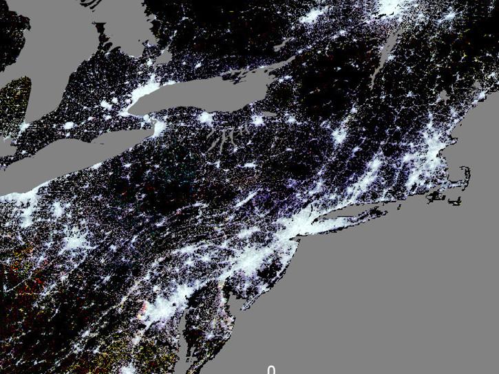
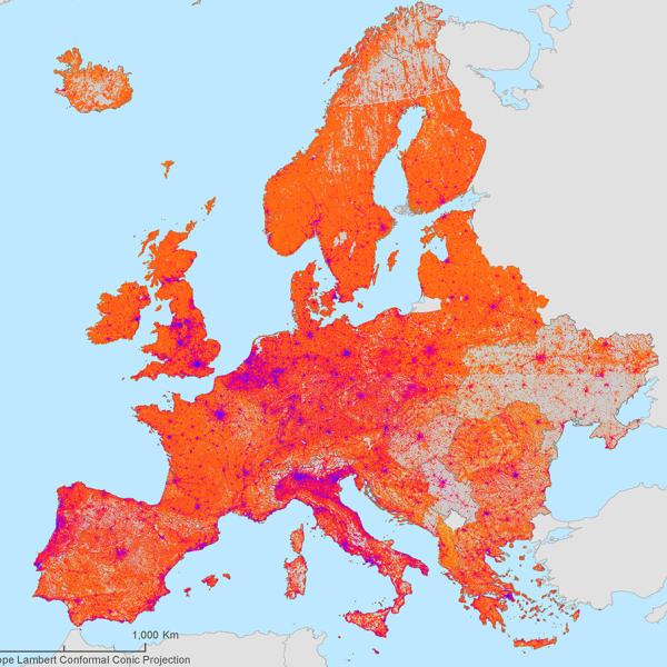
Through Sustainable Development Goal (SDG) 11, the UN proposes to make cities inclusive, safe, resilient, and sustainable. A critical part of this SDG Goal is monitoring urban sprawl and access to green and public spaces as well as monitoring air quality in urban areas. NASA Earth observations can aid in assessing progress towards meeting these objectives.
Image
The world has seen a general increase in urbanization (the amount of built-up area per person) over the past 20 years, according to the United Nations (UN), which notes that "...the share of land allocated to streets and open spaces...averaged only about 16 per cent globally. Of those, streets accounted for about three times as much urban land as open public spaces." Open green spaces are vitally important for maintaining the physical and mental health and well-being of communities.
Through Sustainable Development Goal (SDG) 11, the UN proposes to make cities inclusive, safe, resilient, and sustainable. A critical part of this SDG Goal is monitoring urban sprawl and access to green and public spaces as well as monitoring air quality in urban areas. NASA Earth observations can aid in assessing progress towards meeting these objectives.
The Earth Observations Toolkit for Sustainable Cities and Communities is an online knowledge resource for countries and cities interested in applying Earth observations to support their SDG 11 monitoring and urban policy planning and implementation needs. Key toolkit components include links to data, tools, and various use cases. The toolkit also aims to facilitate engagement among local communities, cities, national agencies, and Earth observation experts, and promote knowledge sharing and collaboration between cities and countries.
Image
Urban sprawl in Las Vegas, NV, from 8 July 1985 (left image) to 21 March 2021 (right image). The left image is Web-Enabled Landsat Data (WELD), available from 1984-2001, and the right image is Harmonized Landsat Sentinel-2 (HLS), available from 2020 to present. These images can be interactively explored in NASA Worldview. Image: NASA Worldview.
SDG Goals are divided into broad Targets that are further divided into Indicators used to track progress toward accomplishing Targets. NASA provides measurements of air quality, land surface reflectance, land cover, population, and other socioeconomic data that provide metrics for tracking progress toward meeting SDG Targets. The data and resources in this Pathfinder are specifically related to SDG 11 Targets 11.1, 11.3, 11.6, and 11.7 (described below). In addition, the Disasters Data Pathfinder can be used in providing information related to SDG 11 Target 11.5 (reduce the impact from disasters).
SDG Goal 11: Make cities inclusive, safe, resilient, and sustainable
Target 11.1: By 2030, ensure access for all to adequate, safe and affordable housing and basic services and upgrade slums.
Indicator 11.1.1: Proportion of urban population living in slums, informal settlements, or inadequate housing.
Target 11.3: By 2030, enhance inclusive and sustainable urbanization and capacity for participatory, integrated and sustainable human settlement planning and management in all countries.
Indicator 11.3.1: Ratio of land consumption rate to population growth rate.
Target 11.6: By 2030, reduce the adverse per capita environmental impact of cities, including by paying special attention to air quality and municipal and other waste management.
Indicator 11.6.2: Annual mean levels of fine particulate matter (e.g. PM2.5 and PM10) in cities (population weighted).
Target 11.7: By 2030, provide universal access to safe, inclusive and accessible, green and public spaces, in particular for women and children, older persons and persons with disabilities.
Indicator 11.7.1: Average share of the built-up area of cities that is open space for public use for all, by sex, age, and persons with disabilities.
The NASA datasets listed in the following sections help measure progress toward meeting the above SDG 11 Targets. While not designed to be a complete list of all salient resources available through NASA's Earth science collection, the following information about NASA data, products, and services will help you chart a path to finding the information you need.
Please visit the Earthdata Forum, where you can interact with other users and NASA subject matter experts on a variety of Earth science research and applications topics.
Data on uptake of land by urbanized land uses, which often involves conversion of land from non-urban to urban functions, and changes in land cover from deforestation, etc.
Data to monitor air pollutants locally, regionally, and globally and to further determine the risk for health conditions or diseases that are exacerbated by poor air quality and the locations that might be impacted.
Other Resources
NASA ARSET Training
NASA's ARSET, which is part of the NASA Applied Sciences Capacity Building Program Area, trains people to use Earth-observing data for environmental management and decision-making. ARSET training programs relevant to this SDG are:
Earth Observations for Monitoring the UN Sustainable Development Goals aims to show the potential and current applications of Earth observations and geospatial information for monitoring the UN SDGs. This training shows participants how to access, interpret, and apply NASA Earth observations to local and global scales, with a focus on applying Earth observations to address SDG monitoring and reporting.
Introduction to Population Grids and their Integration with Remote Sensing Data for Sustainable Development and Disaster Management focuses on the different global population grids and their application to a range of topics related to development planning and monitoring of the SDGs (e.g., environment, hazards, and access to resources). Participants learn about the latest data and methods used to produce global grids, how the grids incorporate remote sensing inputs, and how population grids can be used in conjunction with other types of data.
The POPGRID Data Collaborative aims to bring together and expand the international community of data providers, users, and sponsors concerned with georeferenced data on population, human settlements, and infrastructure.
Trends.Earth is a platform from CI for monitoring land change using Earth observations in an innovative desktop and cloud-based system. Trends.Earth allows users to plot time series of key indicators of land change (including degradation and improvement), to produce maps and other graphics that can support monitoring and reporting, and to track the impact of sustainable land management or other projects.
Earthdata Search is a tool for data discovery of Earth Observation data collections from NASA's Earth Observing System Data and Information System (EOSDIS), as well as U.S and international agencies across the Earth science disciplines.
Users (including those without specific knowledge of the data) can search for and read about data collections, search for data files by date and spatial area, preview browse images, and download or submit requests for data files, with customization for select data collections.
Image
In the project area, for some datasets, users can customize granules. Users can reformat the data and output as HDF, NetCDF, ASCII, KML, or GeoTIFF format, and can choose from a variety of projection options. Data can be subset to obtain only the bands that are needed.
Image
Panoply
HDF and NetCDF files can be viewed in Panoply, a cross-platform application that plots geo-referenced and other arrays. Panoply offers additional functionality, such as slicing and plotting arrays, combining arrays, and exporting plots and animations.
Giovanni is an online environment for the display and analysis of geophysical parameters. There are many options for analysis. The following are the more popular ones:
Time-averaged maps are a simple way to observe the variability of data values over a region of interest.
Map animations are a means to observe spatial patterns and detect unusual events over time.
Area-averaged time series are used to display the value of a data variable that has been averaged from all the data values acquired for a selected region for each time step.
Histogram plots are used to display the distribution of values of a data variable in a selected region and time interval.
Data recipe for downloading a Giovanni map as NetCDF and converting its data to quantifiable map data in the form of latitude-longitude-data value ASCII text
Worldview
NASA's Worldview visualization application provides the capability to interactively browse over 950 global, full-resolution satellite imagery layers and then download the underlying data. Many of the available imagery layers are updated within three hours of observation, essentially showing Earth as it looks "right now." This supports time-critical application areas such as wildfire management, air quality measurements, and flood monitoring. Imagery in Worldview is provided by NASA's Global Imagery Browse Services (GIBS). Worldview also includes nine geostationary imagery layers from GOES-East, GOES-West, and Himawari-8 available at ten minute increments for the last 30 days. These layers include Red Visible, which can be used for analyzing daytime clouds, fog, insolation, and winds; Clean Infrared, which provides cloud top temperature and information about precipitation; and Air Mass RGB, which enables visualization of specific air mass types (e.g., dry air, moist air, etc.). These full disk hemispheric views allow for almost real-time viewing of changes occurring around most of the world.
Image
AppEEARS
AppEEARS at LP DAAC offers a simple and efficient way to access and transform geospatial data from a variety of federal data archives. AppEEARS enables users to subset geospatial datasets using spatial, temporal, and band/layer parameters. Two types of sample requests are available: point samples for geographic coordinates and area samples for spatial areas via vector polygons.
Performing Area Extractions
After requesting an area extraction, users are taken to the Extract Area Sample page where they specify a series of parameters that are used to extract data for the areas of interest.
Spatial Subsetting
Define the region of interest in one of three ways:
Upload a vector polygon file in shapefile format (a single file with multiple features or multipart single features can be uploaded). Files in .shp, .shx, .dbf, or .prj format must be zipped into a file folder to upload.
Upload a vector polygon file in GeoJSON format (users can upload a single file with multiple features or multipart single features).
Draw a polygon on the map by clicking on the Bounding box or Polygon icons (single feature only).
Select the date range for the time period of interest.
Specify the range of dates for which data are desired for extraction by entering a start and end date (MM-DD-YYYY) or by clicking on the Calendar icon and selecting dates a start and end date in the calendar.
Adding Data Layers
Enter the product short name (e.g., MOD09A1, ECO3ETPTJPL), keywords from the product long name, a spatial resolution, a temporal extent, or a temporal resolution into the search bar. A list of available products matching the query will be generated. Select the layer(s) of interest to add to the Selected layers list. Layers from multiple products can be added to a single request. Be sure to read the list of available products available through AppEEARS.
Image
Selecting Output Options
Two output file formats are available:
GeoTIFF
NetCDF4
If GeoTIFF is selected, one GeoTIFF will be created for each feature in the input vector polygon file for each layer by observation. If NetCDF4 is selected, outputs will be grouped into files in .nc format by product and by feature.
Image
Interacting with Results
From the Explore Requests page, click the View icon to view and interact with results. This will take users to the View Area Sample page.
The Layer Stats plot provides time series boxplots for all of the sample data for a given feature, data layer, and observation. Each input feature is renamed with a unique AppEEARS ID (AID). If the feature contains attribute table information, users can view the feature attribute table data by clicking on the Information icon to the right of the Feature dropdown. To view statistics from different features or layers, select a different aid from the Feature dropdown and/or a different layer of interest from the Layer dropdown.
Image
Please see the AppEEARS documentation to learn more about downloading the output as files in GeoTIFF or NetCDF4 format.
With the Global Subset Tool, users can request a subset for any location on Earth that as GeoTiff or text format, including interactive time-series plots and more. Users specify a site by entering the site's geographic coordinates and the area surrounding that site, from one pixel up to 201 x 201 km. From the available datasets, users can specify a date and then select from MODIS Sinusoidal Projection or Geographic Lat/Long. You will need to register for an Earthdata Login request data.
With the Fixed Sites Subsets Tool, users can download pre-processed subsets for more than 3,000 field and flux tower sites for validation of models and remote sensing products. The goal of the Fixed Sites Subsets Tool is to prepare summaries of selected data products for the community to characterize field sites. It includes sites from networks such as National Ecological Observatory Network, Forest Global Earth Observatory network, Phenology Camera network, and Long Term Ecological Research network.
With the Web Service, users can retrieve subset data (in real time) for any location, time period, and area programmatically using a REST web service. Web service client and libraries are available in multiple programming languages, allowing integration of subsets into a workflow.
Image
Spatial Data Access Tool (SDAT)
The ORNL DAAC’s SDAT is an Open Geospatial Consortium standards-based Web application to visualize and download spatial data in various user-selected spatial/temporal extents, file formats, and projections. Several data sets including land cover, biophysical properties, elevation, and selected ORNL DAAC archived data are available through SDAT. KMZ files are also provided for data visualization in Google Earth.
Within SDAT, select a dataset of interest. Upon selection, the map service will open displaying the various measurements, with the associated granule, and a visualization of the selected granule.
Image
You can then select your spatial extent, projection, and output format for downloading.
Image
Sentinel Toolbox
The ESA Sentinel-1 Mission consists of two satellites, Sentinel-1A and -1B, with synthetic aperture radar instruments operating at a C-Band frequency. They orbit 180° apart, together imaging the entire Earth every six days. SAR is an active sensor and so can penetrate cloud cover and vegetation canopy and can observe at night. Therefore, it is ideal for flood inundation mapping. It also provides useful information to detect movement of Earth material after an earthquake, volcanic eruption or landslide. SAR data are very complex to process, but ESA has developed a Sentinel-1 Toolbox to aid with processing and analysis of Sentinel-1 data.
Before choosing data, it’s important to determine which band meets your needs, as radar signals penetrate deeper as the sensor wavelength increases. This difference in penetration is due to the dielectric properties of a given medium, which dictate how much of the incoming radiation scatters at the surface, how much signal penetrates into the medium, and how much of the energy gets lost to the medium through absorption.
Image
SAR signal penetration by sensor wavelength λ. Image: NASA SAR Handbook.
Note that for biomass estimation, L-band and P-band sensors are preferred over higher frequencies and smaller wavelengths for two reasons: 1) at these bands, the radar waves or energy can penetrate the tree canopy and scatter from larger woody components of the forest, and 2) the scattering from larger tree components, unlike leaves, are more stable temporally and remain highly coherent over the acquisition period in the case of repeated measurements for change detection or interferometric applications (adapted from SAR Handbook, 2019).
The C-band can be used for low-vegetation biomass such as grasslands, shrublands, sparse woodlands, young secondary regeneration, and low-density wetlands.
Another important parameter to take into consideration when choosing a dataset is the polarization, or the direction in which the signal is transmitted and/or received: horizontally or vertically. Dual polarization, for example, refers to two different signal directions, horizontal/vertical and vertical/horizontal (HV and VH). Knowing the polarization from which a SAR image was acquired is important, as signals at different polarizations interact differently with objects on the ground, affecting the recorded radar brightness in a specific polarization channel.
Image
Strong scattering in HH indicates a predominance of double-bounce scattering (e.g., stemmy vegetation, manmade structures), while strong VV relates to rough surface scattering (e.g., bare ground, water), and spatial variations in dual polarization indicate the distribution of volume scatterers (e.g., vegetation and high-penetration soil types such as sand or other dry porous soils). Image: NASA SAR Handbook.
SAR data are complex, requiring a certain level of processing skill.
Once you have downloaded the needed SAR data, it must be calibrated to account for distortion in the data. The objective in performing calibration is to create an image where the value of each pixel is directly related to the backscatter of the surface. So calibration takes into account radiometric distortion, signal loss as the wave propagates, saturation, and speckle. This process is critical for analyzing images quantitatively; it is also important for comparing images from different sensors, modalities, processors, and different acquisition dates.
Image
Important note: DO NOT unzip the downloaded SAR file. Open the .zip file from within the Sentinel Toolbox. When you expand the Bands folder, you will see an amplitude and an intensity file for each polarization option. (The intensity band is a virtual one and is the square of the amplitude.) Open the amplitude file. Subset the data by zooming in to the area of interest and right-clicking on “Spatial Subset from View.”
Calibration is done by following these steps:
Radiometric calibration is performed by selecting Radar/Radiometric/Calibration (leave parameters as default).
Geometric correction is done next to fix the main geometric distortions, due to Slant Range, Layover, Shadow, and Foreshortening. Terrain correction can be performed by selecting Radar/Geometric/Terrain Correction/ Range-Doppler Terrain Correction. This requires a digital elevation model (within the processing parameters, SRTM is the default selection). You can also specify a map projection in the processing parameters.
Image
Another characteristic of SAR images that must be accounted for is speckle. Speckle is the grey level variation that occurs between adjacent resolution cells, creating a grainy texture. Within the Toolbox, speckle can be removed by selecting “Radar/Speckle Filtering/Single Product Speckle Filter,” and then choosing a type of filter; “Lee” is one of the most common.
Image
Change Detection
One approach for monitoring change detection, caused by forest degradation or deforestation, is the log-ratio scaling method. You will need two images for which you have completed the steps above. The images must be from the same season. This is important for change detection operations as it avoids seasonal changes and focuses on true environmental changes in a change detection analysis.
For further information on SAR change detection, see ASF DAAC's change detection recipe for QGIS or change detection recipe for ArcGIS. The SERVIR SAR Handbook also contains tutorials on change detection, developing time series and making RGB composites; these are provided as Python scripts in Jupyter notebooks.
Image
Another option for change detection is to create an RGB composite. When creating RGB composites using SAR data, the example color-scheme is often used. Note that for forest applications in particular, it is always useful to assign cross-polarized (HV/VH) data to the green band as these data are more related to volume scattering of the canopies. Co-polarized data (VV or HH) are suited for the red band, where surface scattering components are more pronounced. When only dual-polarimetric data are available (HH/HV or VV/VH), a color SAR image is often constructed by assigning the ratio of co-polarized to cross-polarized data to the blue channel. For more information on this procedure, read the SAR Handbook Chapter 3.
Image
Sentinel-1 C-band dual polarimetric VV and VH data: (a) VV, (b) VH, (c) VV/VH ratio, and (d) SAR false color composite with RGB = VV/VH/ratio channel assignment. Image acquired on May 31, 2018. Image: NASA SAR Handbook.